- Introduction
- Addressing a Range
- Indirect & R1C1 Notation
- Finding a column
- Using INDIRECT
- Putting it all together
Columns can move, and when using complex formulas (such as importrange), this can lead to problems. Here is how to address a column by its header value, rather than it’s position.
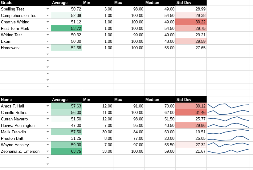
The example google sheet above (populated with random generated test data) is also a generic template that you can use right now to analyse your own data.
Introduction
Writing easy to use, robust and customisable spreadsheets is a challenge, particularly if the people using your spreadsheets are not confident in writing their own custom formulas. You might be importing data from a Google form responses sheet, or providing a summary analysis of a detailed dataset - both of which rely on being able to successfully address the correct columns. What happens if those columns move around? Or you want to be able to just type in the column header and generate data analysis for that column, without having to worry about column letters?
Addressing a Range
Referencing, or addressing, a range normally requires simply selecting the relevant number of cells, be they a small group or entire row/column. When cells move around (rows/columns are inserted or removed), the reference is normally updated without you needing to do anything.
When using the importrange function to bring in data from another sheet, this doesn’t happen automatically, particularly if you are using a static cell reference (e.g. just importing a couple of columns). You might also want to give the option of providing data analysis for a particular row or column, based upon the selection made by a user (e.g. for a particular data point or data subject).
In these more complex cases, you can use an alternate approach by matching the column (or row) header and then return the data for that particular range.
Indirect & R1C1 Notation
Indirect is a vital function when you need to resolve some more complicated range addressing problems. It allows you to build your range address dynamically using the concatenate function, and also to use the alternate R1C1 style of cell notation.
What is R1C1?
R1C1 is an alternate way of addressing spreadsheet cells. Instead of using the traditional letters to indicate which column you are referring to (A-ZZ) you use a number. The R specifies that the number that follows it refers to the row you are addressing (starting at 1) and the C indicates that the number refers to a column (again, starting at 1). So, R1C1 refers to the same cell as A1. The notation is more verbose (which is why it isn’t used as standard), but it is incredibly useful because numbers are a lot easier to handle in formulas.
Using R1C1
While Excel allows you to switch to R1C1 notation globally, Sheets does not have that functionality. Instead, you can use this notation with the Indirect function by passing false as the second parameter.
INDIRECT("R1C1", false)The formula above with give you the value in cell A1 (first row and first column), and the table below gives some equivalent range addresses in both A1 and R1C1 notation.
| A1 Notation | R1C1 Notation | Description |
|---|---|---|
| A1 | R1C1 | Cell in the first row and first column (A) |
| B2 | R2C2 | Cell in the second row and second column (B) |
| C:C | R1C3:C3 | All the cells in the third column (C) |
| 4:4 | R4C1:R4 | All the cells in the fourth row |
| 4:4 | R4C1:R4 | All the cells in the fourth row |
| B4:4 | R4C2:R4 | All the cells in the fourth row starting from the second column (B) |
| E3:F | R3C5:C6 | All the cells in the fifth and sixth columm (E & F) starting from the third row |
Finding a column
This is actually fairly easy using match. All we need to do is find our column name (which could be a cell value, like A2 in the example below, or an actual string) in the range of possible column name headings (the first row in this example).
MATCH($A2, $1:$1, 0)MATCH("End of Year Test", $1:$1, 0)In these match formulas, we supply 0 as the third parameter to indicate that we want an exact match. The function itself will either return the position where the header name was found (the column number) or an error if the column wasn’t found.
Using INDIRECT
To reference the entire column, we need to concatenate the column number into an R1C1 formula for indirect, shown below.
INDIRECT("Data!R1C"&MATCH($A2,$1:$1,0)&":C"&MATCH($A2,$1:$1,0), false)This formula will return the contents of the entire column, matching the header specified in cell A2.
Putting it all together
Instead of just displaying the values from a particular column, we can pass all that range data into another aggregating function, such as average.
IFERROR(IF(LEN($A2)>0,AVERAGE(INDIRECT("R1C"&MATCH($A2,$1:$1,0)&":C"&MATCH($A2,$1:$1,0), false)),),)We can also add in a length check using len (to make sure there is a value in cell A2) and wrap the whole formula in an error handler in case the column name is mistyped. This makes a robust formula to address a column, regardless of its position, just by supplying the header name (or form field, in the case of Google Forms).
Related ► Google Calendars on the Web (01 Sep 2018), Protecting Data with Google Drive (14 Aug 2018), Dealing with confidential information in schools (24 Jul 2018)